Data Science
- 1401 words
- 8 minutes to read
Data science and machine learning
During four years of work in data science and astrophysics, I was involved a number of different projects which I managed with limited supervision. The first project analysed gravitational-wave data produced by numerical-relativity simulations of neutron star mergers along with associated equation of state parameters. The aim was to generate the gravitational-wave signal given the equation of state information. The following work was mostly performed using Python with scipy, numpy, and pandas libraries. The data visualisation was performed with a combination of matplotlib and pandas libraries. The Bayesian inference work was performed on a local computer and using High Performance Computing using Slurm.
Parameter estimation using Bayesian inference
During my work at Monash University, I was fortunate to have the opportunity to contribute to the early development of the Bilby Bayesian inference package, Bilby Pypi, Bilby Gitlab.
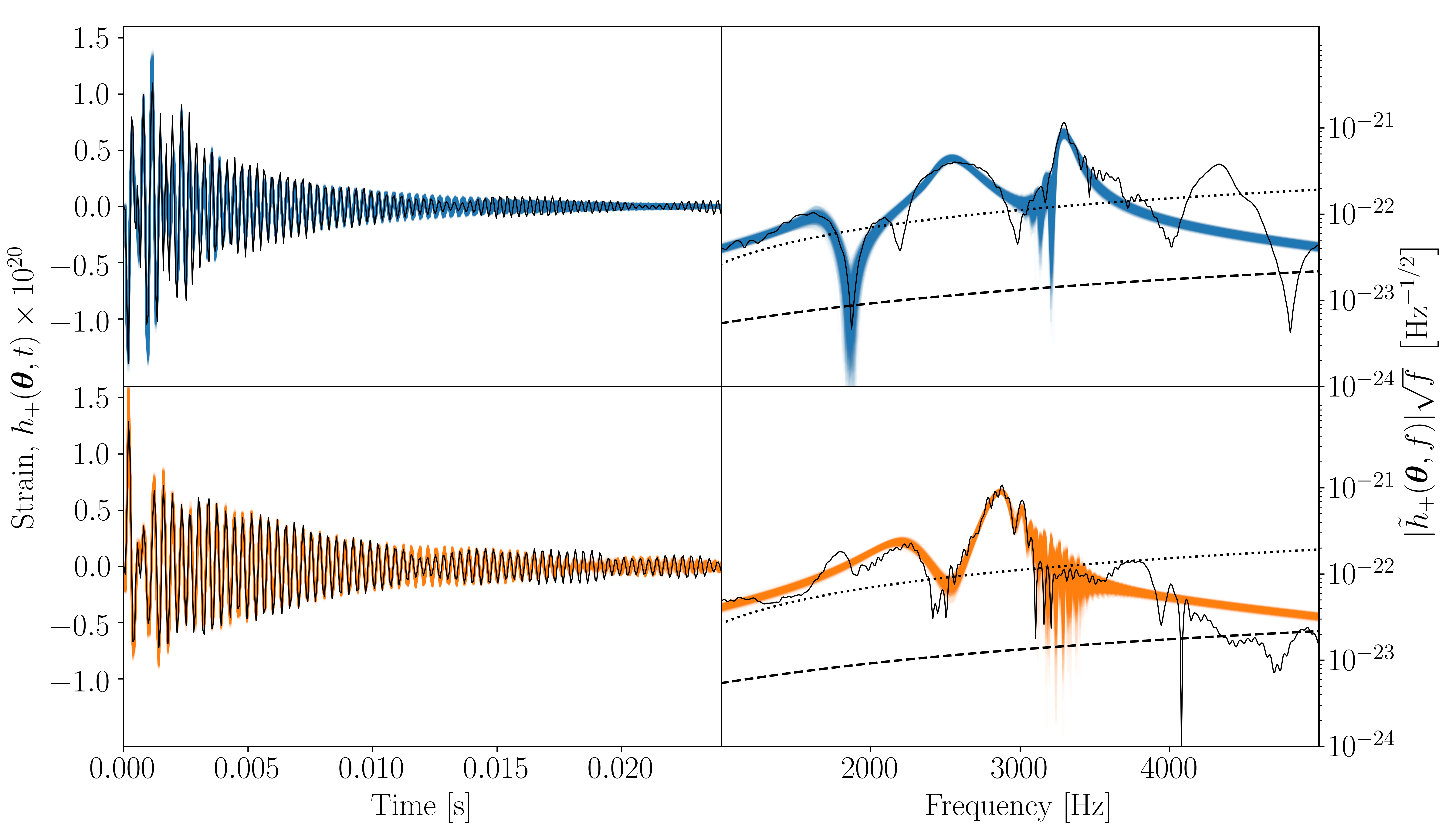
I subsequently used Bilby to perform parameter estimation on gravitational-wave signals using two signal models that I developed. This work is published in Physics Review D 102.043011, arXiv 2006.04396, and Chapter three of my PhD Thesis. Numerical-relativity simulations predict that the gravitational waves emitted immediately after the merging of two neutron stars consist of three main frequency peaks which may drift slightly in frequency. I developed a model based on this prediction and performed parameter estimation of the predicted gravitational-wave signals. The model is a third order exponentially-damped sinusoid with a frequency drift term and see the above publications for the model details.
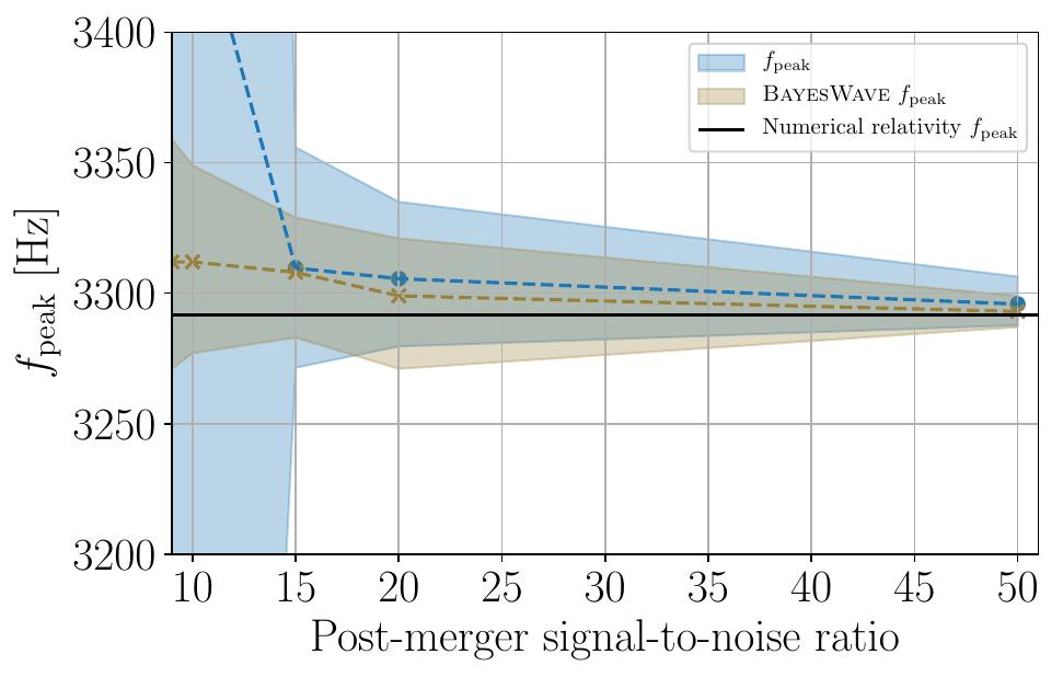
The first plot shows two different gravitational-wave signals in four subplots. The first gravitational-wave signal is shown in the upper subplots and the second in the lower subplots. The left subplots show the time domain gravitational-wave signal and the right subplots show the corresponding frequency-domain signal. In each subplot, the black signals are the true values and the shaded signals are the values predicted from the model.The second plot shows the inference of the main frequency, $f_{peak}$, for different signal-to-noise ratios. The prediction of my model is shown in blue and is contrasted against the BayesWave inference. BayesWave is a model agnostic inference tool that is used in the gravitational wave community.
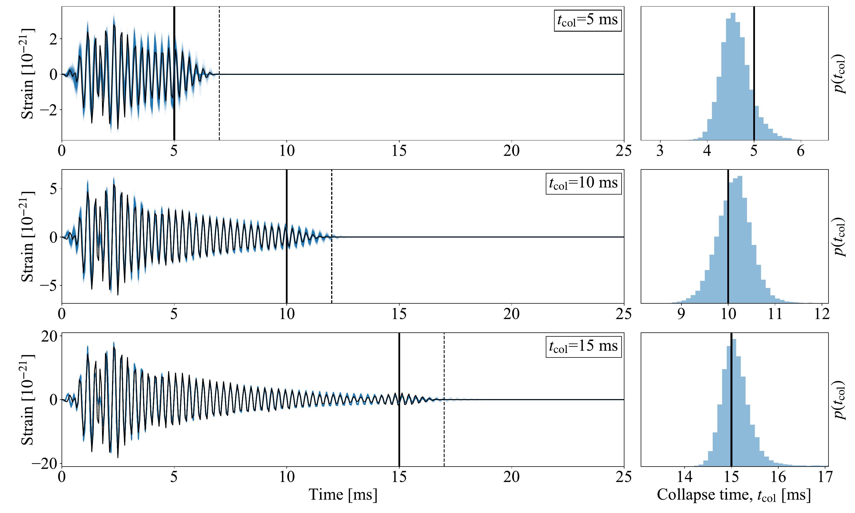
The above signal model was extended to measure the collapse time of the signal. This work was published in arXiv 2106.04064, and Chapter four of my PhD Thesis. The following plot shows the predicted gravitational-wave signals with different collapse times. The left subplots show the time-domain signal and the right subplots show the inferred collapsed time.
Hierarchical machine learning model
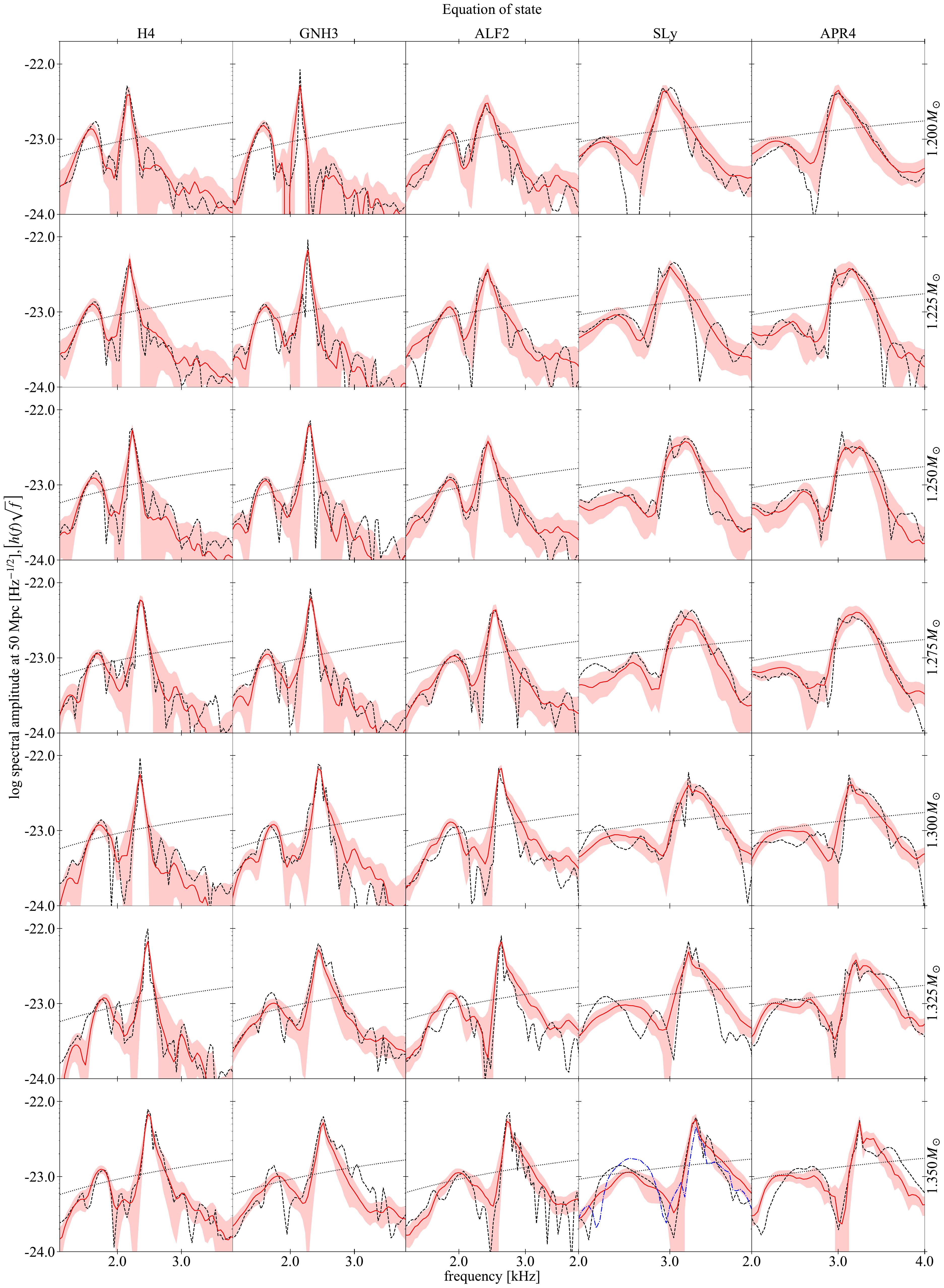
We developed a multi-layered machine learning algorithm that was trained to produce gravitational-wave spectra. This investigation followed on from an earlier analysis using Principal Component Analysis, and Random Forest and Lasso regressors. We had a relatively small data set with 35 time-domain signals. Each of these waveforms were associated with system parameters on which we based our model. Of the thirteen system parameters, we found that we could achieve good results using Leave-One-Out Cross-Validation by using only three system parameters. The results were published in Physics Review D 100.043005, arXiv 1811.11183 and Chapter two of my PhD Thesis. The following plot shows how well I was able to reconstruct the cross-validated spectrum for a given signal.
The model parameters are $(C, K, M)$ and the gravitational-wave signal is $H(f)$. The multiple layers in the algorithm consist of:
1. Preprocess all gravitational-wave signals by converting to the frequency domain and performing a frequency shift to align the peak frequencies. The resulting signals are designated as H(f).

2. Remove signal under test and associated parameters from the training set.

3. Train analytical relationship between parameters in the training set, this allows C to be determined given (K, M).

4. Train the main model that relates the system parameters (C, K, M) to the signals H(f) where C is calculated from step 3. After training H(f) can be predicted given (K, M).

5. The inferred spectra is frequency shifted by an analytical relationship that relates K and fpeak.

6. Compare the predicted H(f) to the value in the test set. This is what is shown in the plot above.
Principal Components Analysis and Random Forest Regression
In these projects, I analysed gravitational-wave time-domain signals in both the time domain and frequency (Fourier) domain. Summaries of these results are shown below, for more details refer to my honours thesis. The main methods used were principal components analysis, random forest regression, and lasso regression.
Principal Component Analysis
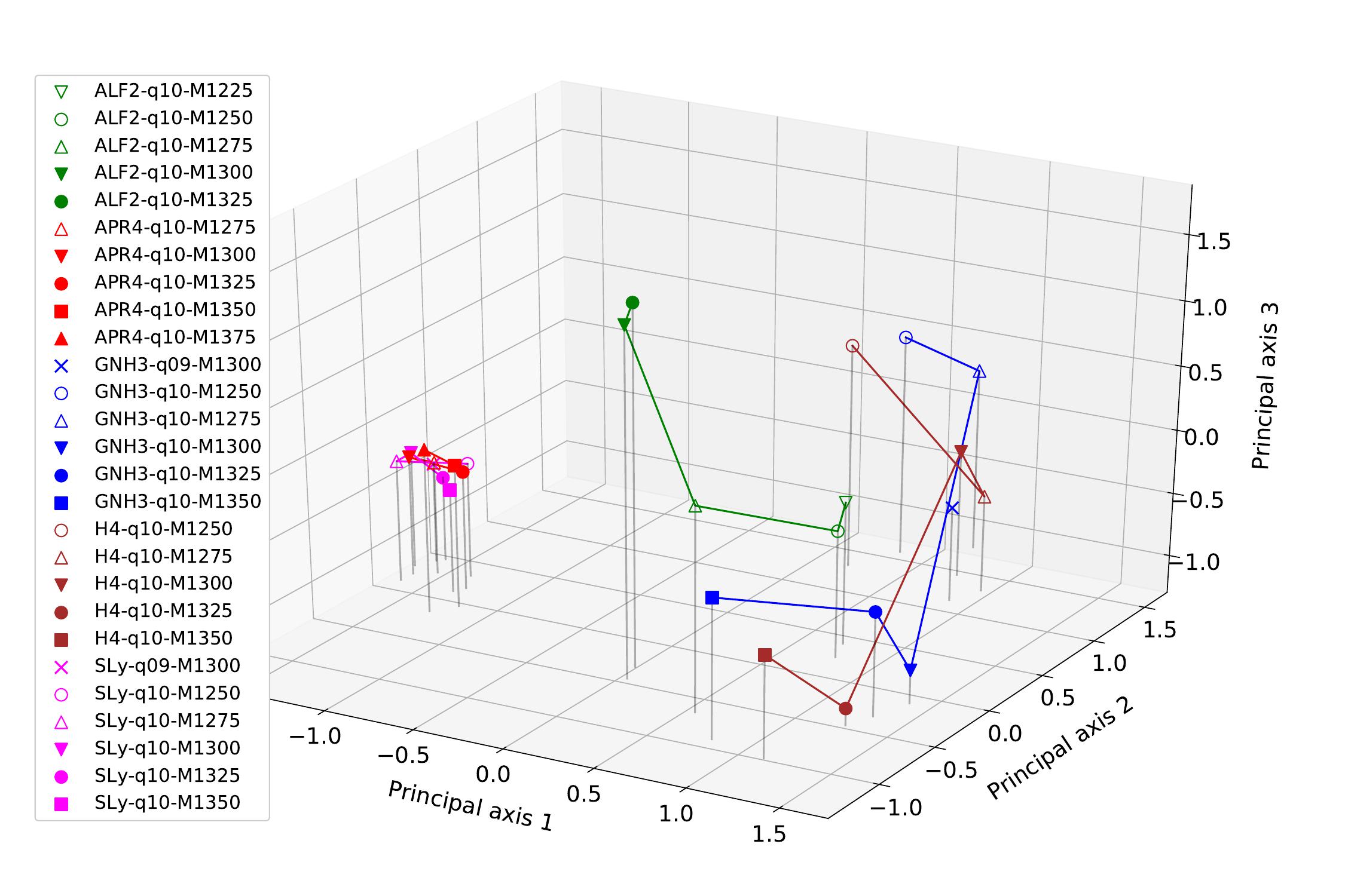
For unsupervised learning, I used principal component analysis to investigate the grouping of signals in respect to the principal components. The data was naturally separated into five different categories which are shown by colour on the plots below. The first plot shows the principal components when reduced to the three most significant components, and the second plot shows the projection of this plot onto the first two principal components. As can be seen from both of these plots, the APR4 (red) and SLy(pink) have similar principal components and are clustered closely in these projections. The other signals are loosely clustered together in another part of the parameter space.
Random Forest
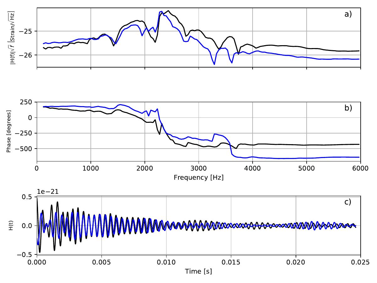
For supervised learning, I implemented random forest regression to predict the time domain signal given a number of neutron star parameters. This was performed in the frequency domain with the intention of predicting a time domain signal. The following plot shows the amplitude and phase of the original signal in black, followed by the leave-one-out cross-validated prediction in blue. The bottom trace shows the time domain signals for both. The right hand plot shows the relative importance of each parameter determined from the random forest decision trees. At face value, it appears that the first four parameters: $\bar{R}, \bar{k}_{2}, J, M_{b}$, account for around 50% of the variance due to parameters, however this is not the whole story, as there are correlations between a number of parameters which has not been shown here.
